The coronavirus outbreak has caused a devastating effect on people all around the world and has infected millions.
The exponential escalation of the spread of the disease makes it emergent for appropriate screening methods to detect the
disease and take steps in mitigating it. The conventional testing technique involves the use of Reverse-Transcriptase
Polymerase Chain Reaction (RT-PCR). Due to limited sensitivity it is more prone to providing high false negative rates. Also
due to a high turnaround time (6-9 hours) and a high cost, an alternative approach for screening is called for. Chest
radiographs are the most frequently used imaging procedures in radiology. They are cheaper compared to CT scans and are
more readily available and accessible to the public. Application of advanced artificial intelligence (AI) techniques coupled with
radiological imaging can be helpful for the accurate detection of this disease. In this projecct we will study how state of the art model - EfficientNetB7 is applied to the problem of classification.
To check out my research paper on this work please refer to the following url:
os.listdir('/content/gdrive/My Drive/Final XRAY')['models', 'TEST', 'TRAIN']
%reload_ext autoreload
%autoreload 2
%matplotlib inline
Next up we will import all the necessary libraries. We will use the fastai library which consists of various state of the art pretrained models for image classification and a lot of utilitarian tools which make deep learning easier with less lines of code!
from fastai import *
from fastai.vision import *
import matplotlib.pyplot as plt
import numpy as np
from sklearn import metrics
from fastai.callbacks import *
EfficientNets
With the rise of transfer learning, the essentiality of scaling has been deeply realised for enhancing the performance as well as efficieny of models. Traditionaly scaling can be done in three dimensions viz. depth, width and resolution in terms of convolutional neural networks. Depth scaling pertains to increasing the number of layers in the model, making it more deeper; width scaling makes the model wider (one possible way is to increase the number of channels in a layer) and resolution scaling means using high resolution images so that features are more fine-grained. Each method applied individually has some drawbacks such as in depth scaling we have the problem of vanishing gradients and in width scaling the accuracy saturates after a point and there is a limit to increasing resolution of images and a slight increase doesnt result in significant improvement of performance. Hence Efficientnets are proposed to deal with balancing all dimensions of a network during CNN scaling for getting improved accuracy and efficieny. The authors proposed a simple yet very effective scaling technique which uses a compound coefficientto uniformly scale network width, depth, and resolution in a principled way. We used the pytorch wrapper for efficientnets. To install run the following command:
pip install efficientnet-pytorch

import warnings
warnings.filterwarnings('ignore')
Now we will define an ImageDataBunch which gets our image data into DataLoaders over which our models can be fit. We use the from_folder function to get the images from our folder which is subdivided into Train and Test folders. For image transformations we use the get_transforms function which performs various augmentations on our images viz rotation, , horizontal flip, vertical flip, zooming, warping, affine transformation etc.
The input target size of the images is defined as 224 since most models are compatible with this size including efficientnets. We maintain a Batch Size of 32 in order to ensure efficient usage of memory.
path = '/content/gdrive/My Drive/Final XRAY'
np.random.seed(44)
data = ImageDataBunch.from_folder(path, train="TRAIN", valid ="TEST",
ds_tfms=get_transforms(), size=(224,224), bs=32, num_workers=4).normalize()data.classes, data.c(['COVID', 'NON-COVID', 'PNEUMONIA'], 3)
data.train_dsLabelList (1482 items)
x: ImageList
Image (3, 224, 224),Image (3, 224, 224),Image (3, 224, 224),Image (3, 224, 224),Image (3, 224, 224)
y: CategoryList
COVID,COVID,COVID,COVID,COVID
Path: /content/gdrive/My Drive/Final XRAY
data.valid_dsLabelList (217 items)
x: ImageList
Image (3, 224, 224),Image (3, 224, 224),Image (3, 224, 224),Image (3, 224, 224),Image (3, 224, 224)
y: CategoryList
COVID,COVID,COVID,COVID,COVID
Path: /content/gdrive/My Drive/Final XRAY
We can visualize our Training data in the following cell.
The train and validation split of the respective images is as follows.
Split COVID-19 NO-FINDINGS PNEUMONIA
Training Set 454 610 418
Testing Set 41 94 82
data.show_batch(rows=3, figsize=(10,10))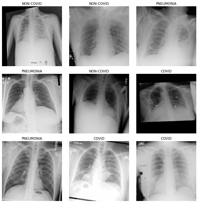
import efficientnet_pytorch
from efficientnet_pytorch import EfficientNet
We will use EfficientNetB7 for training.
model = EfficientNet.from_pretrained('efficientnet-b7')Loaded pretrained weights for efficientnet-b7
To better capture the essence of the performance of the model, along with traditional metrics we use the top2 accuracy which is predicted true for each image if the actual label of the image falls in the top 2 softmax probabilities of the model.
top_5 = partial(top_k_accuracy, k=2)

learn = Learner(data, model, metrics=[accuracy, top_5, error_rate], loss_func=LabelSmoothingCrossEntropy(), callback_fns=[ShowGraph, ReduceLROnPlateauCallback]).to_fp16()learn.fit_one_cycle(4)| epoch | train_loss | valid_loss | accuracy | top_k_accuracy | error_rate | time |
|---|---|---|---|---|---|---|
| 0 | 2.795816 | 11.563503 | 0.382488 | 0.820276 | 0.617512 | 01:03 |
| 1 | 1.872262 | 4.012103 | 0.483871 | 0.852535 | 0.516129 | 01:03 |
| 2 | 1.540921 | 1.864752 | 0.705069 | 0.935484 | 0.294931 | 01:03 |
| 3 | 1.356434 | 1.389227 | 0.834101 | 1.000000 | 0.165899 | 01:02 |
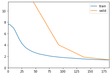
learn.recorder.plot_losses()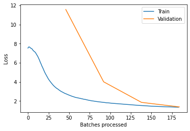
learn.recorder.plot_metrics()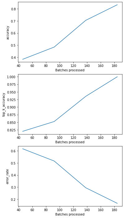
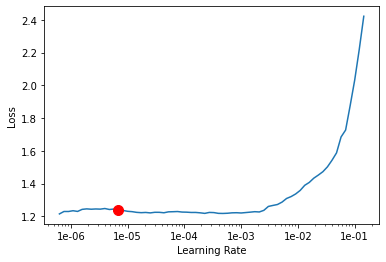
Fastai comes with a very important utility of finding an appropriate learning rate and then fine tuning our models later with the set learning rate. This boosts the performance of the models significantly.
learn.unfreeze()
learn.lr_find()
learn.recorder.plot(suggestion = True)| epoch | train_loss | valid_loss | accuracy | top_k_accuracy | error_rate | time |
|---|---|---|---|---|---|---|
| 0 | 1.218536 | #na# | 00:55 |
LR Finder is complete, type {learner_name}.recorder.plot() to see the graph.
Min numerical gradient: 6.92E-06
Min loss divided by 10: 6.31E-08
learn.fit_one_cycle(100, max_lr=slice(6.82e-6))
| epoch | train_loss | valid_loss | accuracy | top_k_accuracy | error_rate | time |
|---|---|---|---|---|---|---|
| 0 | 1.211556 | 1.233234 | 0.921659 | 1.000000 | 0.078341 | 01:03 |
| 1 | 1.222816 | 1.172435 | 0.940092 | 1.000000 | 0.059908 | 01:03 |
| 2 | 1.244095 | 1.147769 | 0.944700 | 1.000000 | 0.055300 | 01:03 |
| 3 | 1.220592 | 1.137416 | 0.949309 | 1.000000 | 0.050691 | 01:03 |
| 4 | 1.212929 | 1.136014 | 0.949309 | 1.000000 | 0.050691 | 01:02 |
| 5 | 1.207222 | 1.140133 | 0.949309 | 1.000000 | 0.050691 | 01:03 |
| 6 | 1.212577 | 1.142727 | 0.949309 | 1.000000 | 0.050691 | 01:03 |
| 7 | 1.209110 | 1.148496 | 0.949309 | 1.000000 | 0.050691 | 01:03 |
| 8 | 1.213428 | 1.153768 | 0.944700 | 1.000000 | 0.055300 | 01:03 |
| 9 | 1.212053 | 1.158563 | 0.944700 | 1.000000 | 0.055300 | 01:03 |
| 10 | 1.207630 | 1.160250 | 0.944700 | 1.000000 | 0.055300 | 01:02 |
| 11 | 1.210703 | 1.161393 | 0.940092 | 1.000000 | 0.059908 | 01:02 |
| 12 | 1.210255 | 1.163532 | 0.940092 | 1.000000 | 0.059908 | 01:03 |
| 13 | 1.210563 | 1.162763 | 0.940092 | 1.000000 | 0.059908 | 01:03 |
| 14 | 1.199785 | 1.161451 | 0.944700 | 1.000000 | 0.055300 | 01:02 |
| 15 | 1.204878 | 1.165974 | 0.940092 | 1.000000 | 0.059908 | 01:02 |
| 16 | 1.200078 | 1.163577 | 0.944700 | 1.000000 | 0.055300 | 01:03 |
| 17 | 1.196592 | 1.163785 | 0.944700 | 1.000000 | 0.055300 | 01:02 |
| 18 | 1.191627 | 1.167737 | 0.940092 | 1.000000 | 0.059908 | 01:01 |
| 19 | 1.196668 | 1.164468 | 0.940092 | 1.000000 | 0.059908 | 01:01 |
| 20 | 1.193052 | 1.161262 | 0.944700 | 1.000000 | 0.055300 | 01:02 |
| 21 | 1.192981 | 1.164138 | 0.944700 | 1.000000 | 0.055300 | 01:02 |
| 22 | 1.184990 | 1.163553 | 0.944700 | 1.000000 | 0.055300 | 01:02 |
| 23 | 1.190937 | 1.170372 | 0.940092 | 1.000000 | 0.059908 | 01:02 |
| 24 | 1.186672 | 1.174670 | 0.940092 | 1.000000 | 0.059908 | 01:02 |
| 25 | 1.170076 | 1.174799 | 0.940092 | 1.000000 | 0.059908 | 01:02 |
| 26 | 1.174368 | 1.171321 | 0.940092 | 1.000000 | 0.059908 | 01:02 |
| 27 | 1.166383 | 1.174107 | 0.940092 | 1.000000 | 0.059908 | 01:02 |
| 28 | 1.174226 | 1.177173 | 0.940092 | 0.995392 | 0.059908 | 01:02 |
| 29 | 1.170711 | 1.176359 | 0.940092 | 0.995392 | 0.059908 | 01:02 |
| 30 | 1.162668 | 1.175813 | 0.944700 | 1.000000 | 0.055300 | 01:02 |
| 31 | 1.162512 | 1.178215 | 0.944700 | 1.000000 | 0.055300 | 01:02 |
| 32 | 1.168516 | 1.180676 | 0.940092 | 1.000000 | 0.059908 | 01:02 |
| 33 | 1.146605 | 1.181284 | 0.944700 | 1.000000 | 0.055300 | 01:02 |
| 34 | 1.154101 | 1.174066 | 0.949309 | 0.995392 | 0.050691 | 01:03 |
| 35 | 1.159191 | 1.185242 | 0.944700 | 0.995392 | 0.055300 | 01:01 |
| 36 | 1.149488 | 1.187768 | 0.944700 | 0.995392 | 0.055300 | 01:03 |
| 37 | 1.145655 | 1.181144 | 0.944700 | 0.995392 | 0.055300 | 01:02 |
| 38 | 1.152014 | 1.185391 | 0.944700 | 0.995392 | 0.055300 | 01:02 |
| 39 | 1.153827 | 1.186132 | 0.944700 | 0.995392 | 0.055300 | 01:02 |
| 40 | 1.146247 | 1.193885 | 0.944700 | 0.995392 | 0.055300 | 01:02 |
| 41 | 1.143121 | 1.197211 | 0.940092 | 0.995392 | 0.059908 | 01:02 |
| 42 | 1.135645 | 1.209570 | 0.930876 | 0.995392 | 0.069124 | 01:02 |
| 43 | 1.135074 | 1.196061 | 0.935484 | 0.995392 | 0.064516 | 01:02 |
| 44 | 1.151849 | 1.193242 | 0.935484 | 0.995392 | 0.064516 | 01:02 |
| 45 | 1.134802 | 1.188756 | 0.940092 | 0.995392 | 0.059908 | 01:02 |
| 46 | 1.138158 | 1.192837 | 0.935484 | 0.995392 | 0.064516 | 01:02 |
| 47 | 1.129135 | 1.186649 | 0.944700 | 1.000000 | 0.055300 | 01:03 |
| 48 | 1.133389 | 1.193150 | 0.944700 | 1.000000 | 0.055300 | 01:02 |
| 49 | 1.125778 | 1.191461 | 0.944700 | 1.000000 | 0.055300 | 01:02 |
| 50 | 1.131475 | 1.198874 | 0.935484 | 1.000000 | 0.064516 | 01:03 |
| 51 | 1.141228 | 1.205654 | 0.935484 | 1.000000 | 0.064516 | 01:03 |
| 52 | 1.129196 | 1.201473 | 0.935484 | 1.000000 | 0.064516 | 01:02 |
| 53 | 1.134563 | 1.200921 | 0.935484 | 1.000000 | 0.064516 | 01:03 |
| 54 | 1.127136 | 1.202468 | 0.935484 | 1.000000 | 0.064516 | 01:03 |
| 55 | 1.125550 | 1.201220 | 0.940092 | 1.000000 | 0.059908 | 01:03 |
| 56 | 1.117874 | 1.212310 | 0.930876 | 1.000000 | 0.069124 | 01:03 |
| 57 | 1.118835 | 1.209787 | 0.935484 | 1.000000 | 0.064516 | 01:02 |
| 58 | 1.140433 | 1.212276 | 0.935484 | 1.000000 | 0.064516 | 01:03 |
| 59 | 1.125858 | 1.208665 | 0.940092 | 1.000000 | 0.059908 | 01:02 |
| 60 | 1.112389 | 1.208547 | 0.940092 | 1.000000 | 0.059908 | 01:02 |
| 61 | 1.117704 | 1.207139 | 0.940092 | 1.000000 | 0.059908 | 01:03 |
| 62 | 1.115862 | 1.201950 | 0.940092 | 1.000000 | 0.059908 | 01:03 |
| 63 | 1.114401 | 1.203300 | 0.940092 | 1.000000 | 0.059908 | 01:02 |
| 64 | 1.104069 | 1.210942 | 0.940092 | 1.000000 | 0.059908 | 01:03 |
| 65 | 1.111491 | 1.204915 | 0.940092 | 1.000000 | 0.059908 | 01:03 |
| 66 | 1.111911 | 1.203857 | 0.940092 | 1.000000 | 0.059908 | 01:03 |
| 67 | 1.106273 | 1.206619 | 0.940092 | 1.000000 | 0.059908 | 01:02 |
| 68 | 1.111764 | 1.205026 | 0.940092 | 1.000000 | 0.059908 | 01:02 |
| 69 | 1.104027 | 1.209384 | 0.935484 | 1.000000 | 0.064516 | 01:03 |
| 70 | 1.096211 | 1.209802 | 0.935484 | 1.000000 | 0.064516 | 01:03 |
| 71 | 1.104607 | 1.211365 | 0.935484 | 1.000000 | 0.064516 | 01:02 |
| 72 | 1.101600 | 1.207773 | 0.940092 | 1.000000 | 0.059908 | 01:02 |
| 73 | 1.105587 | 1.210494 | 0.935484 | 1.000000 | 0.064516 | 01:03 |
| 74 | 1.099172 | 1.213641 | 0.935484 | 1.000000 | 0.064516 | 01:02 |
| 75 | 1.101368 | 1.213647 | 0.935484 | 1.000000 | 0.064516 | 01:02 |
| 76 | 1.101365 | 1.209697 | 0.935484 | 1.000000 | 0.064516 | 01:02 |
| 77 | 1.111905 | 1.212039 | 0.935484 | 1.000000 | 0.064516 | 01:02 |
| 78 | 1.097285 | 1.214438 | 0.935484 | 1.000000 | 0.064516 | 01:03 |
| 79 | 1.098992 | 1.217427 | 0.935484 | 1.000000 | 0.064516 | 01:04 |
| 80 | 1.110196 | 1.219014 | 0.935484 | 1.000000 | 0.064516 | 01:02 |
| 81 | 1.110621 | 1.218604 | 0.935484 | 1.000000 | 0.064516 | 01:03 |
| 82 | 1.103908 | 1.217055 | 0.935484 | 1.000000 | 0.064516 | 01:04 |
| 83 | 1.103807 | 1.217934 | 0.935484 | 1.000000 | 0.064516 | 01:03 |
| 84 | 1.106353 | 1.220562 | 0.935484 | 1.000000 | 0.064516 | 01:03 |
| 85 | 1.102028 | 1.218156 | 0.935484 | 1.000000 | 0.064516 | 01:03 |
| 86 | 1.098312 | 1.219447 | 0.935484 | 1.000000 | 0.064516 | 01:03 |
| 87 | 1.100400 | 1.220807 | 0.935484 | 1.000000 | 0.064516 | 01:03 |
| 88 | 1.099732 | 1.220042 | 0.935484 | 1.000000 | 0.064516 | 01:03 |
| 89 | 1.098915 | 1.219582 | 0.935484 | 1.000000 | 0.064516 | 01:03 |
| 90 | 1.093679 | 1.217780 | 0.935484 | 1.000000 | 0.064516 | 01:03 |
| 91 | 1.096850 | 1.215652 | 0.935484 | 1.000000 | 0.064516 | 01:02 |
| 92 | 1.098493 | 1.219773 | 0.935484 | 1.000000 | 0.064516 | 01:03 |
| 93 | 1.098292 | 1.217808 | 0.935484 | 1.000000 | 0.064516 | 01:03 |
| 94 | 1.098705 | 1.219644 | 0.935484 | 1.000000 | 0.064516 | 01:02 |
| 95 | 1.091730 | 1.222525 | 0.935484 | 1.000000 | 0.064516 | 01:03 |
| 96 | 1.093058 | 1.221992 | 0.935484 | 1.000000 | 0.064516 | 01:03 |
| 97 | 1.100906 | 1.220918 | 0.935484 | 1.000000 | 0.064516 | 01:04 |
| 98 | 1.100290 | 1.222682 | 0.935484 | 1.000000 | 0.064516 | 01:03 |
| 99 | 1.108818 | 1.222131 | 0.935484 | 1.000000 | 0.064516 | 01:03 |
interp = ClassificationInterpretation.from_learner(learn)
interp.plot_confusion_matrix(title='Confusion matrix')probs,targets = learn.get_preds(ds_type=DatasetType.Valid) # Predicting without TTA
probs = np.argmax(probs, axis=1)
correct = 0
for idx, pred in enumerate(probs):
if pred == targets[idx]:
correct += 1
accuracy = correct / len(probs)
print(len(probs), correct, accuracy)
from sklearn.metrics import confusion_matrix
np.set_printoptions(threshold=np.inf) # shows whole confusion matrix
cm1 = confusion_matrix(targets, probs)
print(cm1)
from sklearn.metrics import classification_report
y_true1 = targets
y_pred1 = probs
target_names = ['Covid-19', 'No_findings', 'Pneumonia']
print(classification_report(y_true1, y_pred1, target_names=target_names))import matplotlib.pyplot as plt
plt.figure()
plt.plot(fpr, tpr, color='darkorange', label='ROC curve (area = %0.2f)' % roc_auc)
plt.plot([0, 1], [0, 1], color='navy', linestyle='--')
plt.xlim([-0.01, 1.0])
plt.ylim([0.0, 1.01])
plt.xlabel('False Positive Rate')
plt.ylabel('True Positive Rate')
plt.title('Receiver operating characteristic (DenseNet 169) ')
plt.legend(loc="lower right")