
How does google understand how to translate ‘今日はどうですか?’ to ‘How are you doing today?’ or vice versa? How do we get to predict a disease spread such as COVID-19 way into the future beforehand? How do automatic Text generation or Text Summarization mechanisms work? The answer is Recurrent Neural Networks. RNNs have been the solution to deal with most problems in Natural language Processing and not only NLP but in Bio-informatics, Financial Forecasting, Sequence modelling etc. To this date, RNNs along with its variants GRUs and LSTMs are used in various state-of-the-art systems for their efficiency in modelling sequential data. In this post we will take a glimpse at how RNNs work in the background by making our RNN model learn how to automatically evaluate a mathematical equation and obtain an answer.
What is a Recurrent Neural Network?
In a traditional feed-forward neural network we can only used a fixed sized input data in which the information moves only in one direction i.e from the input layer to the hidden layer and from there to the output layer. One flavor of feed forward neural network which accepts a fixed input size is the Convolutional Neural Network which is very good in capturing spatially dependent features for eg. Nose features in a face or cat whiskers in an image of a cat. While CNNs and Feed forward networks are very good in capturing spatial features, there seldom is a scope for such data to be seen out there in the wild. Most data in the nature is of a sequential nature. Consider audio signals or textual data or Time series data. This kind of data is variable in size and hence normal feed-forward networks fail to capture the essence of such data as they do not deal with past memory. In order to capture the essence of the entire sequence of data we need to have a mechanism that captures the essence of the previous data and reinforces the contextual representation as we move along the sequence.
Hence come RNNs to the rescue.

The main difference is in how the input data is taken in by the model.
Traditional feed-forward neural networks take in a fixed amount of input data all at the same time and produce a fixed amount of output each time. On the other hand, RNNs do not consume all the input data at once. Instead, they take them in one at a time and in a sequence. At each step, the RNN does a series of calculations before producing an output. The output, known as the hidden state, is then combined with the next input in the sequence to produce another output. This process continues until the model is programmed to finish or the input sequence ends.
Still confused? Don’t anguish yet. Being able to visualize the flow of an RNN really helped me understand when I started on this topic.

As we can see, the calculations at each time step consider the context of the previous time steps in the form of the hidden state. Being able to use this contextual information from previous inputs is the key essence to RNNs’ success in sequential problems.
While it may seem that a different RNN cell is being used at each time step in the graphics, the underlying principle of Recurrent Neural Networks is that the RNN cell is actually the exact same one and reused throughout.
Processing RNN Outputs?
You might be wondering, which portion of the RNN do I extract my output from? This really depends on what your use case is. For example, if you’re using the RNN for a classification task, you’ll only need one final output after passing in all the input - a vector representing the class probability scores. In another case, if you’re doing text generation based on the previous character/word, you’ll need an output at every single time step.

This is where RNNs are really flexible and can adapt to your needs. As seen in the image above, your input and output size can come in different forms, yet they can still be fed into and extracted from the RNN model.
For the case where you’ll only need a single output from the whole process, getting that output can be fairly straightforward as you can easily take the output produced by the last RNN cell in the sequence. As this final output has already undergone calculations through all the previous cells, the context of all the previous inputs has been captured. This means that the final result is indeed dependent on all the previous computations and inputs.
For the second case where you’ll need output information from the intermediate time steps, this information can be taken from the hidden state produced at each step as shown in the figure above. The output produced can also be fed back into the model at the next time step if necessary.
Of course, the type of output that you can obtain from an RNN model is not limited to just these two cases. There are other methods such as Sequence-To-Sequence translation where the output is only produced in a sequence after all the input has been passed through. The diagram below depicts what that looks like.
Now we’ve had enough theory, lets get our hands dirty!
You can find the complete code here at this link
The flow of implementation will be the following.
import numpy as np
import torch
import torch.nn as nn
import torch.optim as optim
from termcolor import coloredprint(f'Using Pytorch Version - {torch.__version__}')
Next up we will synthetically generate sequences of expressions using random numbers generated from 1–100 and use it to train our model and evaluate it.
We define the set of all characters that can be potentially fed to our model. These include the numbers 0–9 and the operators ‘+’ and ‘-’. Note that all characters will be input as a string and the output label will also be a string.
Textual data to numeric data.
Unlike humans, Neural Networks do not do very well with textual input data. In order to leverage the mathematical power of Neural Networks we have to convert them into a numerical format or a numerical encoding that quantifies a particular character or maps a character to a numerical format. There are various formats in which this numerical mapping can be done — Bag of words representation, Tf-idf vectors, One hot vectors and the newest and most effective method i.e Word Embeddings. Since the scale of our problems is not large and the vocabulary size is small we can make do with One hot vector representations to encode our data.
We will use a character_to_index dictionary to get the index at which the character resides and an index_to_character dictionary which maps an index to the encoded character. We will use these dictionaries alternatively while encoding and decoding our input sequence.
`all_chars = '0123456789+-'
num_features = len(all_chars)
char_to_index = {c : i for i, c in enumerate(all_chars)}
index_to_char = {i : c for i, c in enumerate(all_chars)}
print(f'Number of features : {len(all_chars)}')`
We will use the np.random.randint function which is a Pseudo Random Number Generator to generator two number between 0 and 100 and a equal probability distribution of addition and subtraction symbols. We will store the expression as a string and evaluate the expressions and save the results of the evaluations in a string called labels.
def generate_data():
    first_num = np.random.randint(low=0,high=100)
    second_num = np.random.randint(low=0,high=100)
    add = np.squeeze(np.random.randint(low=0, high=100)) > 50.
    if add:
      example = str(first_num) + '+' + str(second_num)
      label = str(first_num+second_num
    else:
      example = str(first_num) + '-' + str(second_num)
      label = str(first_num-second_num)
   return example, label
generate_data()
We represent each token as a more expressive feature vector. The easiest representation for representing a character is one-hot encoding. In this form of representation we take row vectors of size corresponding to the vocabulary size of the characters and mark those indexes as 1 where that character is present in the vocabulary. For example if our input word is ‘GOOD’, the vocabulary size becomes 3 (Set of unique characters) and if the input dictionary is defined as {G : 0, O : 1, D : 2}, we can represent G as [1, 0, 0], O as [0, 1, 0] and D as [0, 0, 1] hence the representation for GOOD will be denoted as
[[1,0,0], [0,1,0] ,[0,1,0], [0,0,1]]
Similarly we will use the decode function to restore our outputs back to the format we intend them to be in. At the end of our Computation we will be left with a vector storing output probabilities of the shape [max_time_steps, num_features] which will store the output evaluation. We take the argmax from each of the row vectors and take the index with the highest probability and convert it into the output expression using our dictionary int_to_char that we previously computed.
def encode(example, label):
 x = np.zeros((max_time_steps, num_features))
 y = np.zeros((max_time_steps, num_features))
 diff_x = max_time_steps - len(example)
 diff_y = max_time_steps - len(label)

 for i, c in enumerate(example):
   x[diff_x+i, char_to_index[c]] = 1
   for i in range(diff_x):
     x[i, char_to_index['0']] = 1
   for i, c in enumerate(label):
     y[diff_y+i, char_to_index[c]] = 1
   for i in range(diff_y):
     y[i, char_to_index['0']] = 1return x, y
def decode(example):
 res = [index_to_char[np.argmax(vec)] for i, vec in enumerate(example)]
 return ''.join(res)def strip_zeros(example): encountered_non_zero = False
 output = ''
 for c in example:
   if not encountered_non_zero and c == '0':
     continue
   if c == '+' or c == '-':
     encountered_non_zero = False
   else:
 encountered_non_zero = True
 output += c
 return output
Generating Batches and Converting to Tensors.
Here we will call the generate function to generate batches of examples and labels and store them in our placeholders.
def create_dataset(num_examples=20000):
 x_train = np.zeros((num_examples, max_time_steps, num_features))
 y_train = np.zeros((num_examples, max_time_steps, num_features))
 for i in range(num_examples):
   e, l = generate_data()
   x, y = encode(e, l)
   x_train[i] = x
   y_train[i] = y
 return x_train, y_train
x_train, y_train = create_dataset(200000)
x_train = torch.from_numpy(x_train)
y_train = torch.from_numpy(y_train)
x_train = torch.tensor(x_train, dtype = torch.float32)
y_train = torch.tensor(y_train, dtype = torch.float32)
device = torch.device('cuda' if torch.cuda.is_available() else 'cpu')
Our Simple RNN model.
Now we come to cream of the project — defining the model for our task!
The nn.Module acts as a Base class for all Neural Network architectures in Pytorch. We will inherit this class to extend our SimpleRNN class. In the constructor of our class we can define some variables that our model will be using such as the hidden dimension size, the number of layers in the RNN cell etc. For our model we will be using one RNN layer followed by a fully connected layer that outputs one single variable at each timestep which shall be passed over a softargmax layer to get the index of the prediction.
We also need to pass an initial hidden state to our RNN cell for initial computation which is initialized to zeros for the first computation.
class SimpleRNN(nn.Module):
  def __init__(self, input_size, output_size, hidden_dim,n_layers):
   super(SimpleRNN, self).__init__()
   self.hidden_dim = hidden_dim
   self.n_layers = n_layers
   self.rnn = nn.RNN(input_size, hidden_dim, n_layers, batch_first = True)
   self.fc1 = nn.Linear(hidden_dim,hidden_dim * 2)
   self.fc2 = nn.Linear(hidden_dim * 2, output_size)
   self.relu = nn.ReLU()

 def forward(self, x):
   batch_size = x.size(0)
   hidden = self.init_hidden(batch_size)
   hidden = hidden.cuda()
   out, hidden = self.rnn(x, hidden)
   out = self.fc1(out)
   out = self.fc2(self.relu(out))
   return out, hidden

def init_hidden(self, batch_size):
  hidden = torch.zeros(self.n_layers, batch_size, self.hidden_dim)
  return hidden
Initializing the model and defining hyperparameters.
After defining the model above, we’ll have to instantiate the model with the relevant parameters and define our hyper-parameters as well. The hyper-parameters we’re defining below are:
- n_epochs : Number of Epochs –> Number of times our model will go through the entire training dataset
- lr : Learning Rate –> Rate at which our model updates the weights in the cells each time back-propagation is done
For a more in-depth guide on hyper-parameters, you can refer to this comprehensive article.
Similar to other neural networks, we have to define the optimizer and loss function as well. We’ll be using CrossEntropyLoss as the final output is basically a classification task and the common Adam optimizer.
model = SimpleRNN(input_size = num_features, output_size = num_features , hidden_dim = 12, n_layers = 1)
model.cuda()
n_epochs = 1000
lr = 0.01
criterion = nn.CrossEntropyLoss()
optimizer = torch.optim.Adam(model.parameters(), lr = lr)
Training the model.
Now we can begin our training! As we only have a few examples, the training process is very fast. However, as we progress, larger datasets and deeper models mean that the input data is much larger and the number of parameters within the model that we have to compute is much more.
This training process involves two processes one is called the Forward Propagation and the other is the Backward Propagation. In the forward propagation the model multiplies the input with the previous hidden state for each time step to finally generate the final hidden state. During the Backward Propagation step the gradients are sent backward by calculating the loss with a given criterion (in this case — the cross entropy loss) and the weights of the model are updated so that the model can make more accurate predictions.
for epoch in range(1, n_epochs + 1):
 optimizer.zero_grad()
 x_train = x_train.cuda()
 output, hidden = model(x_train)
 loss = criterion(output, y_train.cuda())
 loss.backward()
 optimizer.step()
 if epoch % 10 == 0:
   print('Epoch: {}/{}.............'.format(epoch, n_epochs), end=' ')
   print("Loss: {:.4f}".format(loss.item()))
Evaluation.
Let’s test our model now and see what kind of output we will get. As a first step, we’ll define some helper function to convert our model output back to text.
full_seq_acc = 0
for i, pred in enumerate(preds):
 pred_str = strip_zeros(decode(pred))
 y_test_str = strip_zeros(decode(y_test[i]))
 x_test_str = strip_zeros(decode(x_test[i]))
 col = 'green' if pred_str == y_test_str else 'red'
 full_seq_acc += 1/len(preds) * int(pred_str == y_test_str)
 outstring = 'Input: {}, Out: {}, Pred: {}'.format(x_test_str, y_test_str, pred_str)
 print(colored(outstring, col))
 print('\nFull sequence accuracy: {:.3f} %'.format(100 * full_seq_acc))
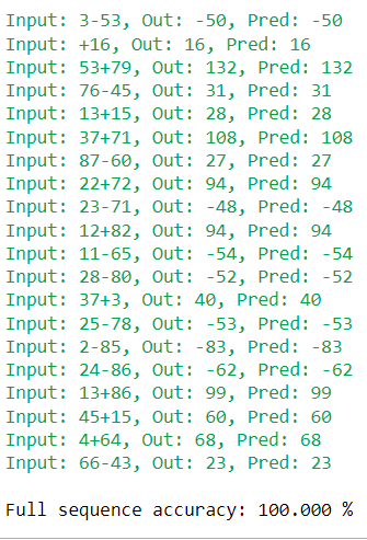
And Voila! We can see a hundred percent accurate results while testing. Thus we have seen the power of Recurrent Neural Networks in sequence modelling. The function of RNNs can be extrapolated to a number of other tasks such as Text Summarization, Text Generation, Time Series Forecasting and much more. Today there are better variants of RNNs namely Gated Recurrent Units and Long Short Term Memory networks which have little tweaks in their architecture to solve two main problems with vanilla RNNs i.e 1. Vanishing and Exploding Gradients and 2. Inability to capture long term sequence dependency. Today with the introduction of the Transformer Architecture even LSTMs and GRUs are outperformed by some of the state of the art variants which make use of the attention mechanism and completely eliminate the use of recurrence. But the good old RNN still remains in use today and has laid a foundation for some of the legendary works in NLP.